I’ve been learning a lot of really interesting stuff about time-series data, lately. Over the past month I’ve learned how to consume Factory IoT sensor data from an MQTT server, process it in StreamSets, persist it in OpenTSDB, visualize it in Grafana, and forecast it with Tensorflow. It’s really amazing how this all fits together. I’m going to focus this blog post on the Tensorflow part.
OpenTSDB REST API examples
OpenTSDB is a specialized database for time-series data. It has a really nice REST API which allows you to create metrics, read metric values, list metrics, etc. I use curl when working with REST APIs. It often takes me some trial-and-error to figure out the proper curl syntax, so here are some examples that should help anyone just getting started with OpenTSDB:
Here’s how to write a random metric value to opentsdb (running on localhost port 4242):
curl -X POST --data '{"metric": "sys.ian.test", "timestamp": '`date +%s`',"value": '$RANDOM',"tags": {"host": "web01","dc": "lga"}}' "http://localhost:4242/api/put"
Here’s how to query OpenTSDB to see what metrics are available. Run this in a web browser, not with curl or wget:
http://localhost:4242/api/suggest?type=metrics&max=10000
Here’s how to query all the time series data for a metric and pretty print json:
curl http://localhost:4242/api/query?start=1h-ago&m=sum:sys.ian.test | jq
For more information about the OpenTSDB REST API, see http://opentsdb.net/docs/build/html/user_guide/query/examples.html.
Forcasting time-series data with RNNs in Tensorflow
Justin Brandenburg, a data scientist with MapR, posted an excellent blog describing how to predict a sequence of time-series values using Recurrent Neural Networks (RNNs). His blog is at https://mapr.com/blog/deep-learning-tensorflow/. He also posted accompanying code, showing the RNN in action with Tensorflow. That code is at https://github.com/JustinBurg/IoT_Predictive_Maintenance_Demo.
The following Jupyter notebook shows how I adapted Justin’s code to predict values for IoT sensor data in OpenTSDB. This notebook is intended to be run with a python3 kernel.
I’ve spent zero time trying to improve the accuracy of this model, so the actual predictions are pretty poor, but since it runs, I’m happy!
Jupyter Notebook
import numpy as np
import pandas as pd
import json
from pandas.io.json import json_normalize
from mapr_streams_python import Consumer, KafkaError
import random
import matplotlib
import matplotlib.pyplot as plt
%matplotlib inline
Pull test data from OpenTSDB
import base64
import requests
import yaml
url="http://nodeb:4242/api/query?start=16h-ago&m=avg:Panel2Power"
headers = {'content-type': 'application/vnd.kafka.v1+json'}
r = requests.get(url, headers=headers)
d = (yaml.safe_load(r.text)[0]['dps'])
df3 = pd.DataFrame(list(d.items()))
df3.columns = ['timestamp', 'value']
df3['timestamp']=pd.to_datetime(df3['timestamp'], unit='s')
df3 = df3.sort_values(by=['timestamp'])
ts = pd.Series(df3['value'].values, index=df3['timestamp'])
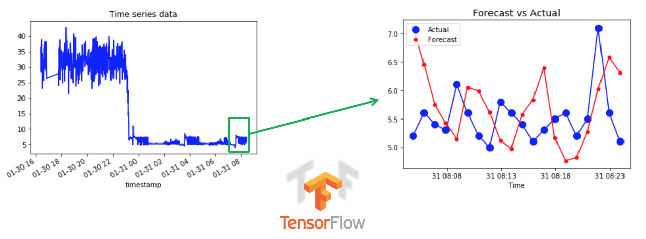
ts.plot(c='b', title="Time series data")
plt.show()
ts.head(10)

Segment the OpenTSDB data into windows
We'll train the RNN model based on a narrow segment of the data recorded in opentsdb.
TS = np.array(ts[0:801])
num_periods = 20
f_horizon = 1

x_data = TS[:(len(TS)-(len(TS) % num_periods))]
x_batches = x_data.reshape(-1, 20, 1)

y_data = TS[1:(len(TS)-(len(TS) % num_periods))+f_horizon]
y_batches = y_data.reshape(-1, 20, 1)
print (len(x_batches))
print (x_batches.shape)
print (y_batches.shape)
def test_data(series,forecast,num_periods):
    test_x_setup = TS[-(num_periods + forecast):]
    testX = test_x_setup[:num_periods].reshape(-1, 20, 1)
    testY = TS[-(num_periods):].reshape(-1, 20, 1)
    return testX,testY
X_test, Y_test = test_data(TS,f_horizon,num_periods)
print (X_test.shape)
import tensorflow as tf
import os
import shutil
import tensorflow.contrib.learn as tflearn
import tensorflow.contrib.layers as tflayers
from tensorflow.contrib.learn.python.learn import learn_runner
import tensorflow.contrib.metrics as metrics
import tensorflow.contrib.rnn as rnn
Build the RNN model in Tensorflow
tf.reset_default_graph()
# num_periods = 20
inputs = 1
hidden = 100
output = 1

x = tf.placeholder(tf.float32, [None, num_periods, inputs])
y = tf.placeholder(tf.float32, [None, num_periods, output])

basic_cell = tf.contrib.rnn.BasicRNNCell(num_units=hidden, activation=tf.nn.relu)
rnn_output, states = tf.nn.dynamic_rnn(basic_cell, x, dtype=tf.float32)
learning_rate = 0.001
stacked_rnn_output = tf.reshape(rnn_output, [-1, hidden])
stacked_outputs = tf.layers.dense(stacked_rnn_output, output)
outputs = tf.reshape(stacked_outputs, [-1, num_periods, output])

loss = tf.reduce_sum(tf.square(outputs - y))
optimizer = tf.train.AdamOptimizer(learning_rate = learning_rate)
training_op = optimizer.minimize(loss)
init = tf.global_variables_initializer()
epochs = 1000

with tf.Session() as sess:
    init.run()
    for ep in range(epochs):
        sess.run(training_op, feed_dict={x: x_batches, y: y_batches})
        if ep % 100 == 0:
            mse = loss.eval(feed_dict={x: x_batches, y: y_batches})
            print (ep, "\tMSE:", mse)

    y_pred = sess.run(outputs, feed_dict={x: X_test})
Compare forecasts with ground truth
plt.title("Forecast vs Actual", fontsize = 14)
timestamps = df3['timestamp'][-len(pd.Series(np.ravel(Y_test))):].values
plt.plot(timestamps, pd.Series(np.ravel(Y_test)), "b-", markersize = 10)
plt.plot(timestamps, pd.Series(np.ravel(Y_test)), "bo", markersize = 10, label="Actual")
plt.plot(timestamps, pd.Series(np.ravel(y_pred)), "r-", markersize = 10)
plt.plot(timestamps, pd.Series(np.ravel(y_pred)), "r.", markersize = 10, label="Forecast")
plt.legend(loc="upper left")
plt.xlabel("Time")

plt.show()

Please provide your feedback to this article by adding a comment to https://github.com/iandow/iandow.github.io/issues/6.
